The Normal Distribution vs. Student’s T-Distribution

An intuitive visualization of why we use t-distributions

Introduction

In this article I attempt to provide an intuitive visualization of why Student’s t-distribution is often used over the normal distribution. Many introductory statistics and data science courses provide a rationale for the use of t-distributions along the lines of it being useful in situations where either the sample size is small and/or the population’s standard deviation is unknown. While correct, the rationale remains abstracted through such an explanation and learners may achieve a more powerful understanding through a clear and simple visualization.

The Normal Distribution

The normal distribution, also sometimes referred to as a bell curve, is one of the most frequently used distributions and often the starting point for learning about distributions in general due to its relative simplicity. Given a mean (μ) and standard deviation (σ), a normal distribution can be modeled with the following probability density function:

The probability density function for a normal distribution

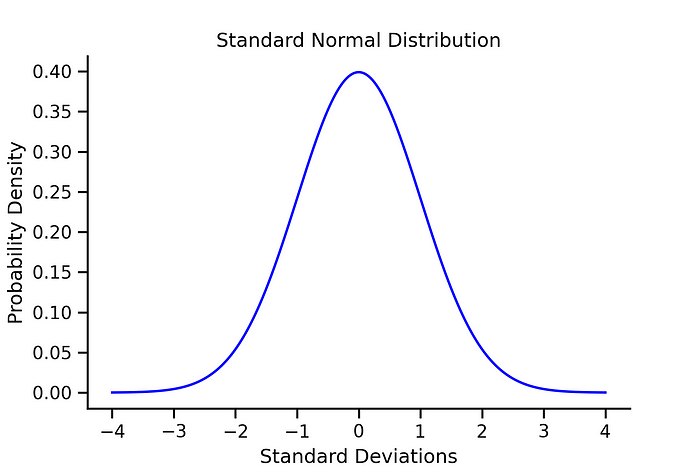
A variety of different Python libraries makes visualizing a normal distribution fairly simple. The code below outputs a graph of a special type of normal distribution called the standard normal distribution — i.e., where the mean is explicitly equal to zero and the standard deviation is explicitly equal to one.

Code:

Explanation:

For those not familiar with Python or programming in general, here’s a quick explanation of what the above code is doing:

• Imports the various libraries used for creating the graph
• Sets x equal to 500 evenly spaced values between -4 and +4
• Sets y equal to the output of the normal distribution probability density function at the values of x
• Specifies the labels and title for the graph and then plots the data
• Includes some optional styling methods to make the output look a bit nicer (sns.despine() removes the top and right borders of the graph)

Output:

Student’s T-Distribution

The t-distribution is similar to the normal distribution in many ways but does not assume knowledge of the population mean and standard deviation the way the normal distribution does. The probability density function of the t-distribution is as follows, where Γ represents the gamma function and ν represents the degrees of freedom:

The probability density function for Student’s t-distribution

Importantly, the degrees of freedom, calculated as one less than the sample size in most situations, has a large impact on the shape of the distribution at lower values. This will be explored a bit further in the comparison section, but for now let’s visualize a t-distribution with a single degree of freedom.

Code:

Explanation:

• The above code is largely the same as in the normal distribution section with slight changes on lines 9 and 11
• Line 9 sets the specified degrees of freedom to the df variable
• Line 11 sets y equal to the output of the t-distribution probability density function at the values of x given the df parameter

Output:

A Visual Comparison

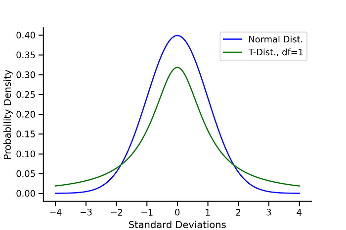
Now that we’ve seen both the standard normal distribution and a t-distribution with a single degree of freedom, let’s plot them together to see how they compare.

Code:

Output:

Key Differences:

With only a single degree of freedom, the t-distribution is much flatter and has fatter tails than the standard normal distribution. The power of the t-distribution comes from its ability to adjust for smaller sample sizes (and therefore less degrees of freedom) by effectively having a more conservative estimate of probability density.

Put another way, the t-distribution adjusts for a natural decrease in confidence at lower sample sizes that the normal distribution does not account for.

At higher degrees of freedom, the t-distribution approximates the normal distribution, making it useful at both small and large sample sizes. The animation below shows a comparison between the t-distribution and the normal distribution at degrees of freedom ranging from 1 to 50.

Conclusion

And there you have it. Not only does Student’s t-distribution not require information regarding the population mean and standard deviation (which are rarely known in real world experiments), but it also has increased flexibility at various sample sizes. These properties make it much more attractive to use over the normal distribution in most instances.

Feedback

Any questions, comments, or other feedback? I’d love to hear from you! Feel free to leave a response or shoot me an email at tjkyner@gmail.com. If you liked this article and want to see more, make sure to leave a 👏.

License

The code and images contained within this article were all produced by myself and are released under the GNU General Public License v3.0.